Introduction
 The emerging markets (EM) local currency sovereign bonds asset class has undergone a period of extraordinary expansion over the last 15 years. The subset of the asset class that is readily accessible to global investors is now composed of 19 countries and has a market value of USD 1,130 billion. Improvements in market depth and breadth has greatly expanded the capacity of EM governments to fund themselves domestically. This has in turn reduced their reliance on foreign currency denominated borrowings. These developments have been concurrent with improved market accessibility for global investors which has led to an increasingly diverse mix of market participants invested in the asset class (JP Morgan, 2018).
Since the financial crisis, central bank quantitative easing has supported capital flows and investment in EM. However, it has also pushed up asset prices, suppressed volatility and potentially induced imbalances that will at some point need to be corrected. The subsequent reversal of these policies by the FED in particular creates an environment in which EM local bond prices can diverge from fundamentals. Therefore, insight into the fundamental drivers of bond valuation is becoming an even more indispensable tool for global investors making asset allocation and trading decisions under these exacting conditions.
Calculating useful fair-value estimates for EM local currency yield curves is challenging. On top of the existing difficulties faced by developed market bond investors, EM issuers have added complexities. They are more credit risky, have less credible inflation management regimes and are subject to additional market frictions. Turkey is a case in point: the central bank’s inflation target has been 5% since 2012 and yet realized inflation has swung between 6% and 15%. Therefore a new model is developed which contributes to the growing body of methodologies on EM local bond valuation by introducing methods that are similar to the credit relative valuation approach. The paper starts with explaining the methodology. Subsequently it is applied to a case study on Polish and Russian local bonds to indicate its usefulness and limitations for investors and traders.
A building-block approach to EM local yield curve valuation
Breaking up the valuation process into components makes the challenge of EM local bond valuation more tractable. For global investors, EM local bond valuation can initially be divided into two parts:
- A fair-value estimate of the local yield curve; and
- The valuation of EM foreign exchange (FX) rates against the investor’s base currency
Valuing emerging markets local currency sovereign bonds is notoriously difficult
This paper explores the former. Currency effects are an important complimentary topic as they form a significant part of the total risk of investing in local currency bonds. However, much has been written elsewhere4 and therefore, this article does not discuss FX valuation.
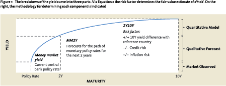
Subsequently, the local yield curve is broken down into three parts, which are valued separately:
- The money market yield;
- The difference between the money market yield and the 2-year bond yield (MM2Y); and
- The difference between the 2-year bond yield and the 10-year bond yield (2Y10Y).
Firstly, it is assumed that the observed money market yield is ‘fair’ given that expected short-term returns on money market investments are very close to current yields. Next, central banks are recognized as having a significant influence on the short end of the yield curve. As such, the fair-value of MM2Y is based on forecasts of the course of overnight rates over the next two years. These forecasts can be based on analyst consensus figures where available, or those of the individual investor.
The last component – the focus of this paper – is the valuation of 2Y10Y. In developed markets, it is well documented (NBIM, 2011) that normally positive 2Y10Y gives rise to positive term premiums that reward investors for taking duration risk in the long run. Lustig (2017) shows that EM local yield curves also generally exhibit positive term premiums, so there is an indication that investors in this asset class are also compensated for taking duration risk. For developed markets, econometric methods can be used to estimate fair-value of term premiums.6 Crucially, these methods depend on some degree of stationarity where economic and market conditions may vary, but in a systematic manner. EM economies can behave erratically and conditions can change suddenly and significantly – due to the result of an election for example – making this kind of statistical analysis less reliable.
For these reasons, an alternative model is developed for the valuation of 2Y10Y. The model has two parts. First a risk factor is defined. It starts with the observed EM bond spread over the most relevant ‘risk-free’ developed market benchmark yield. The 10-year yield is chosen because longer-maturity bonds are more sensitive to uncertainty in underlying risk drivers than shorter-term bonds. Also, bonds with longer maturity are often not available. Key fundamental drivers of the level of 2Y10Y are inflation risk and credit risk. Uncertainty about future inflation dynamics and credit fundamentals increases with the investment horizon. Investors thus ask for additional compensation in longer-maturity bonds vis-à-vis shorter-maturity ones in the form of higher yields.7 2-year bonds are less sensitive to inflation risk and credit risk. The sensitivity to these risks is well-capture by 10-year rates and therefore the model does not incorporate bond yield spreads at shorter maturities.
Quantitative term premium fair-value estimation is most applicable to countries with stable monetary policy and inflation dynamics and a lower exposure to global risk sentiment
Credit risk and inflation risk are represented in the model by subtracting the Credit Default Swap (CDS) premium and the expected inflation differential between the EM and its benchmark country from the aforementioned spread. CDS prices are used rather than other available alternatives, such as USD-denominated bond spreads, as they better reflect the all-in cost of hedging credit risk. The remainder, hereafter referred to as the ‘risk factor’, then provides an indication of the term premium.
Specifically the risk factor is calculated as:
+/+ Yield differential of the local 10Y EM bond with the 10Y reference country bond. Reference country (e.g., US, DE) is chosen based on trade considerations.
–/– 5Y CDS country premium. 5-year contracts are chosen as these have more reliable price data due to higher liquidity, are readily available, and are known to capture countryspecific credit factors in the long run (Csonto and Ivaschenko, 2013).
–/– Inflation differential. Calculated as the difference in one-year-ahead expected inflation between the local market and the reference country.
 Second, the model connects the risk factor with the fair-value estimate of 2Y10Y. If risk factors contain useful information about the fair-value of 2Y10Y then two intertemporal dynamics are to be expected. First, credit and inflation surprises – manifested through changes in the risk factor defined above – may translate to future steepening or flattening of the curve as market prices adjust to changing fundamentals. Second, the curve may steepen or flatten without any changes in risk factors, indicating potential mean reversion over time. The authors’ experience indicates that these dynamics typically manifest over a period of 1 to 12 months, thus a lead-lag relationship between the current risk factor and the future 2Y10Y is expected in that time span. This, in turn, relates the current risk factor with the current fair-value of 2Y10Y, which is assumed to revert to future actual 2Y10Y value within 1 to 12 months. Any difference between fair-value and current value of 2Y10Y gives rise to term risk premiums, which can be positive or negative over time.
The lead-lag relationship between current risk factors and future 2Y10Y is evaluated by crosscorrelations. Per country, the lag that produces the strongest lead-lag relationship is used as the chosen lag in Equation 1. Parameters â and ˆb in Equation 2 are estimated using OLS from Equation 1. Estimation is done on weekly data from Jan 2010 to Dec 2017.
A key finding of the research performed with this model is that quantitative estimation of the fair values of 2Y10Y are best evaluated within the context of the then-actual market circumstances. For this reason, a traditional out-of-sample test – consisting of showing the effectiveness of the model for various countries on various time frames using performance statistics – is not considered. Instead the model is evaluated using out-of-sample case studies.
Figure 1 summarizes the three components of the yield curve and their drivers of fair-value.
Using the identity:

the relationship between the risk factor and the 2Y10Y fair-value is captured by the following model assumption:

Fair-value term premium estimates: the cases of Russia and Poland
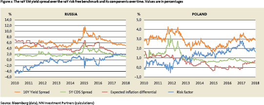 Russia and Poland serve as examples to assess the results of the model. Russia is chosen because over the last few years it has experienced various episodes of economic and political turmoil. In contrast, while Poland has not been immune to the European sovereign debt crisis of the early 2010s, the country remains one of the more resilient and stable EM economies.
Germany is chosen as the Polish reference country because it is its major trading partner. The US is chosen as Russia’s reference country, due to its energy exports. The risk factor and the underlying market data for each country are shown in Figure 2. As the Russian data shows in early 2010, risk factors can be strongly negative as there are no restrictions that would enforce lower or upper bounds. Our explanation in this case is that the Russian curve was overvalued relative to US Treasuries, especially in light of the high inflation. Additionally, because credit risk and inflation risk are not always independent, level and/or scale differences can be introduced by the overlap of these factors. However, the model’s approach to estimating fair-value corrects for this as it is the dynamics of the risk factor that matters when it comes to 2Y10Y estimation, not the average or volatility.
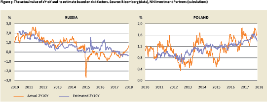 To connect the risk factor with the fair-value of 2Y10Y, first the chosen lag in Equation 1 is established. For Poland, a shift of nine months causes the strongest lead-lag relationship, while for Russia the lag is four months. The analysis shows that i) the lead-lag relationship is statistically significant and ii) much of the variation in the observed 2Y10Y can be explained by past values of risk factors.
Figure 3 shows the evolution of the relationship between the actual 2Y10Y and estimate based on the risk factor for Poland and Russia from 2010 to 2017. The estimate represents the goodness of fit of Equation 1 and Equation 2.
In Poland’s case, the estimated fair-value line captures the trend in the actual 2Y10Y quite well with the observed values oscillating around it. For Russia, prior to 2014, 2Y10Y estimates were lower than observed values, correctly indicating a flattening trend. However, when the Ukraine crisis and subsequent sanctions hit, the quantitative estimate became unreliable. It overlooked the inversion of the curve during the crisis and incorrectly predicted significant steepening after the fact.
Stability of the local market key to usefulness of valuation anchors
An out-of-sample case study covering the first six months of 2018 casts more light on the effectiveness of the valuation methodology. This timeframe is long enough for market corrections to manifest, and short enough for active positioning.
Model fair value estimation can be useful in practice, but is still just one piece of the puzzle when it comes to emerging markets debt investing
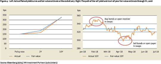 At the end of 2017, the Polish policy rate stood at 150bps. The central bank was dovish as inflation had not yet reached its target level and policy was synchronised with the ECB. Over the next 24 months, the authors expected the central bank to hike 25-50bps to match a pick-up in inflation. Our qualitative fair-value estimate of the 2Y rate based on the average expected hike was thus 187.5bps. The quantitative risk factor-based estimate of 2Y10Y was 140bps. Therefore the fair-value yield of 327.5bps for the 10Y Polish government bond (Figure 4). Throughout a dynamic first half of 2018, the 10Y yield gyrated around this valuation anchor which resulted in the identification of two notable trading opportunities in local bonds or equivalent interest rate swaps (IRS).
Russia’s policy rate was 7.75% at the end of 2017 with inflation well below the 4% target and the market pricing in a series of cuts. There was also a high probability of a negative surprise that could disrupt the central bank’s gradual rates normalization. Thus, the authors projected a near-term cut of 50bps and no cuts thereafter. The fair-value of 2Y10Y was negatively inverted by 25bps, resulting in a yield estimate of 7% for the 10Y bonds. The approach would have suggested adding duration risk at that time, as the bonds were trading 50bps wide.
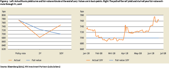 Russian 10Y yields did initially drop to about 7%, only to rise sharply to almost 7.5% in the second quarter of 2018. Therefore the fair-value estimate of the yield turned out to be too low. As the Russian in-sample analysis in the previous section also suggested, when the market is not driven by fundamentals the valuation anchor loses its usefulness.
Our broader research covering 15 local markets indicates that the observations about Poland and Russia are of a more general nature. The valuation methodology is less applicable to countries that do not have a history of managing inflation successfully such as Russia, Brazil and Turkey. Conversely, for countries such as Poland, Korea or Hungary, the model tends to be more accurate. However, when global factors or difficult-to-quantify risks such as politics dominate, the usefulness of our valuation methodology deteriorates. Instead, successful navigation of such markets relies heavily on manager skill and experience.
Valuation supplements – rather than replaces – portfolio management approach
As the importance of EM local currency bond markets increases and market participants become more heterogeneous, the relevance of estimating fair-values for yield curves becomes greater. This article contributes to a growing body of literature on this topic by proposing a methodology to estimate yield curve fair-values, focusing on a quantitative method to indicate fair-values of 2Y10Y. The examples of the Polish and Russian curves also highlight a more general point: in EM there can be added value in using quantitative valuation methods to supplement portfolio management decisions. But investors need to be careful not to place too much reliance on such methods when market sentiment and current events overshadow fundamentals. A multi-faceted approach that utilises both qualitative and quantitative aspects for assessing fundamentals, valuations and sentiment – as well as the skill and judgment to assess the relative importance of these factors – is critical for successfully investing in EM debt.
Literature
- Cochrane, J.H. and Piazessi, M., 2005, Bond Risk Premia, American Economic Review, v95 (1, Mar), 138-160.
- Csonto, B. and Ivaschenko, I., 2013, Determinants of Sovereign Bond Spreads in Emerging Markets: Local Fundamentals and Global Factors vs. Ever-Changing Misalignments, IMF Working Paper No. 164.
- Elton, E. J. et al., 2001, Explaining the Rate Spread on Corporate Bonds, The Journal of Finance VOL. LVI, No. 1, February.
- Emery, T. and Nystedt, J., 2015, Are Emerging Market Foreign Currencies Finally Attractive?, Morgan Stanley Investment Focus.
- JP Morgan, 2018, EM Local Markets Guide (12th edition).
- Ludvigson, S.C. and Ng, S., 2009, Macro Factors in Bond Risk Premia, Review of Financial Studies, Oxford University Press for Society for Financial Studies, vol. 22 (12), 5027-5067.
- Lustig, H. N. and Stathoupolos, A. and Verdelhan A., 2017, The Term Structure of Currency Carry Trade Risk Premia, NBER Working Paper No. 19623.
- Norges Bank Investment Management, 2011, The term premium, NBIM Discussion Note, #4.
- Wright, J.H., 2008, Term Premiums and Inflation Uncertainty: Empirical Evidence from an International Panel Dataset, The Federal Reserve Board Finance and Economics Discussion Series, 2008-25.
Notes
- Lewis Jones, CFA, FRM, is Lead Portfolio Manager Emerging Markets Local Currency Debt at NN Investment Partners. Richard Sanders, CFA, is Strategic Advice Specialist at NN Investment Partners.
- Represented by the JP Morgan GBI-EM Global Index, figures as at June 30th, 2018.
- Central Bank of the Republic of Turkey, June 2018.
- Interested readers can refer to Emery (2015) for commonly-used valuations methodologies.
- For results given below, NNIP monetary policy expectations are used.
- For purely statistical approaches see Cochrane, 2005 or methods that use information related to inflation or growth expectations in Ludvigson, 2009.
- For the effects of inflation on term premium, see Wright (2008). For credit risk effects, see Elton (2001).
- Bloomberg expert panel consensus forecasts. Ticker: ECPI[two-letter country code][last two digits year] Index.
- R2 values are 40% and 48% for Poland and Russia, respectively. Significance, in terms of R2 , does vary in the order of 10%-20% when changing lags with several months for both countries. Regression coefficients (Equation 2) are less dependent on differences in lags. This is observed in general for all 15 local markets considered.
in VBA Journaal door Lewis Jones (l), Richard Sanders (r)
