In this article we will explore the subject of liability driven investments (LDI). FTK regulation in the Netherlands, changes in internal accounting rules (IAS 19) and insurance regulation (Basle II and Solvency II) will force pension funds and insurers to focus on how well their assets are set to meet their liabilities rather than only on asset appreciation. Here, we will talk about the impact on pension funds, but the same problems also face insurance companies.
 Defining the problem in an ALM context
The new set of rules will have a profound impact on the way portfolios are structured: more than ever before the focus of attention for pension managers is on the pension surplus, the assets minus the liabilities of a pension fund. Managers of the assets thus need to be aware of what is going to influence this surplus, both on the asset side and on the liability side. The volatility of the surplus will be driven by asset allocation decisions and the sensitivity of the liabilities to interest rate shifts. Also, pension plan policies regarding inflation compensation and contributions will impact the surplus. Going forward, investment decisions should be measured as a function of marginal risk/return to the surplus, not just on an asset only basis.
Traditional sources of return have relied heavily on market (beta) risk, with a relatively high weighting in equities. Given the higher volatility of equities and the resulting impact on the surplus, it is likely that these traditional sources of return may not be suitable for most pension funds going forward (unless solvency rates are high). In our view, portfolios should be built around four basic concepts:
- Initially, interest rate risk should be hedged to the extent possible
- Beta risk should be added as a function of the overall risk tolerance of the pension fund
- Alpha (the ability to generate excess return versus a given benchmark) should be the main engine of return
- Although inflation is not explicitly part of the solvency calculations, it cannot be ignored as it impacts expected future cash flows.
Let us point out clearly that PIMCO, as an active fixed income manager, is neither an actuarial firm nor an asset allocation specialist. Instead, we work closely with the client and their consultant/actuarial to establish the cash flows going forward and to discuss the impact of asset allocation decisions on the bond portfolio.
Having said this, the fixed income portfolio will by default have to fulfill point number one; equities and other asset classes will have a zero weighting in hedging liabilities and cannot help here. We will pause here and elaborate on how we go about defining an interest rate-hedging portfolio at PIMCO.
LDI Benchmark Modeling at PIMCO
PIMCO’s Analytics Group provides the analytical machinery for LDI Benchmark Solutions. There is no separate LDI Modeling group using different risk analytics tools, rather an effort is made to recast any LDI study in a way that all of PIMCO’s existing analytics tools can be exploited. There are several advantages to this approach, starting with consistency: an LDI solution is analyzed/stress-tested using the same tools that are used on a day-to-day basis to monitor the firm’s existing 1000+ accounts. These tools are used by portfolio managers and financial engineers and are improved based on continuous feedback.
There are three steps in building an LDI solution:
Step 1 Cash Flows as a Security
The Analytics Group computes risk sensitivities (yield curve level, yield curve shape, currency, inflation sensitivity and spread sensitivities) for any security in its portfolios. A stream of cash flows can then be treated like any security with a given cash flow structure, and its profile in terms of the afore mentioned risk sensitivities can be quickly assessed.
Step 2 Building a Benchmark
Given the risk profile of the cash flows, the Analytics Group will build a portfolio of liquid fixed income securities that aims to meet the cash flow requirements as closely as possible. The extent to which the solution can track the cash flows depends on a variety of factors, the main ones being client specifications on securities to be used. For example, a client requiring a maximum of 20% inflation indexation will not be able to hedge inflation as well as a client who is willing to have 50% indexation.
The ultra-long duration profile presents a common problem. A profile with a duration of 20 years or above cannot be duration-hedged even with the longest conventional bond (the longest German Bund, DBR 4 37, has a duration of less than 19 years). In this case some less liquid instruments, like Strips or long Swaps, may help to provide extra duration.
Curve duration can also present a challenge. Typically, a portfolio that contains government bonds will have a steepening bias compared to the cash flows. The bias can be removed by paying swaps in the front end and hedging via receiving swaps in the ten-year sector.
Another possible mismatch coming from the ultralong maturity of the cash flows is convexity. Here as well, use of swaps and derivatives can be extremely helpful to track the cash flows very closely. In all these cases, it is clear that client restrictions on the use of swaps/derivatives/structured products can limit the “fit” of the solution to the cash flows.
The Benchmark’s Performance
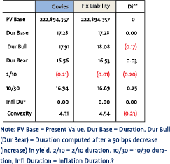
 Once a benchmark is built, mismatches versus the cash flows are summarized in a table like the following model case:
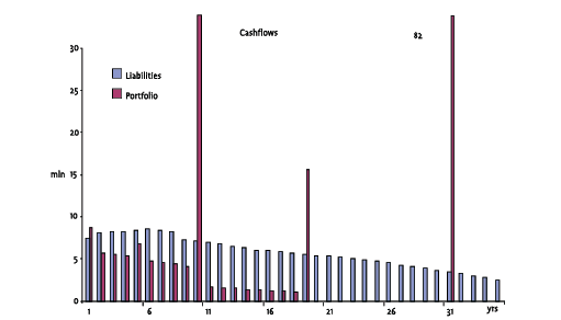
Note how present value and base duration are exactly matched, while the worst mismatches come from 2/10’s, 10/30’s and convexity. The mismatch in 2/10’s and 10/30’s comes from the bullet-type structure of the portfolio: while the liabilities will be smoothly distributed over, say, 50 years, the tracking portfolio will typically consist of not more than 6-7 securities spread over the maturity horizon of the liabilities (see graph below):
Convexity is in general the one risk that is very hard to minimize, as most current securities are not convex enough compared to the liabilities (development of a new 50 year maturity sector could provide the instruments to minimize the convexity mismatch1 ).
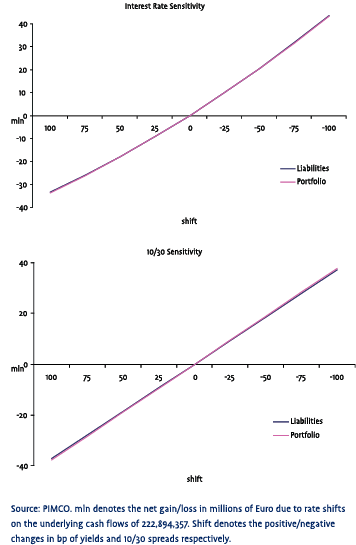
The graphs on the next page show the sensitivity (in millions of EUR) of the benchmark & cash flows to parallel shifts in the term structure and changes in 10/30’s. Note how the cash flows and benchmark are indistinguishable on the first graph - sensitivity to interest rate risk (first graph) is identical for Cash Flows (“Liabilities”) and the Benchmark (“Portfolio”), while there is a slight mismatch at the 10/30’s level (second graph).
 Optimization Techniques
There are two cases:
1. The client allows PIMCO to go short In this case existence/uniqueness of solutions depends on the number of securities chosen – we show this follows from linear algebra. Namely, suppose we are trying to optimize the following 7 measures:
- Base Duration
- Bull Duration
- ear Duration
- 2/10’s
- 0/30’s
- Convexity
- Inflation Duration
We denote the vector containing these numbers for the cash flows by b (b is a 7x1 vector). We will also have a vector of portfolio weights x from which we construct the portfolio. Suppose we do not fix the dimension of the vector x (this amounts to not fixing the number of securities to be used), but just denote its dimension with k. We use A to denote the matrix of risk sensitivities for every security (A is a 7xk matrix). Then our optimization requires the following equation to hold:
 Ax=b.
Ax=b.
The solution will be given by:
x=A-1b
where A-1 denotes the matrix inverse of A. Whether there is a solution, and whether it is unique or not, depends on the dimension of the vector x relative to the vector b. In our case, the dimension of b is 7 (the number of measures to be optimized). It is a fact from linear algebra that if k7, multiple solutions will exist. Translated to our LDI setting, this means:
If the number of securities used for the benchmark is smaller than the number of measures to be optimized, a solution is impossible.
If the number of securities used for the benchmark is equal to the number of measures to be optimized, a unique solution exists.
If the number of securities used for the benchmark is greater than the number of measures to be optimized, many solutions exist.
Given that the number of measures to be optimized is rarely greater than ten, an LDI benchmark will usually not contain more than 10 securities.
2 The client does not allow PIMCO to go short
In this case we cannot use the previous method since the exact solution might require short positions in the portfolio. The no-short conditions are constraints that have to be satisfied by the solution, making it a constrained optimization problem.
Depending on the client’s parameters, the benchmark portfolio will have a very low tracking error versus the liabilities (usually between 10-40 bp). Although this is not the same as a pure cashfor–cash matching, which theoretically could be achieved by matching all future cash flows with swaps, we do believe that the advantages for pension funds are clear:
- There is no need to set up a swap program, which requires documentation, margin regulation and oversight
- Adjustments can be made regularly without altering the structure (in the case of a swap overlay unwinds would have to take place)
- The benchmark portfolio consists of liquid securities, which can be priced on a daily basis and provide a transparent benchmark
It is also worth noting that we tend to avoid long dated zero swaps (e.g. > 40 years) as part of our solution. The reason for this is that the perceived benefit of hedging the duration and convexity risk a bit better will likely be nullified by the pricing risk (long duration zero swaps tend to have very wide bid-offer spreads).
Step3 Incorporating the next steps: beta and alpha
Once we have defined a benchmark portfolio based on the liabilities and hedged the interest rate risk, we can add beta and alpha risk to increase the expected return of the portfolio. Again, this will be a function of the risk budget and the marginal risk/return attribution to the surplus, rather than in asset only context. Given the lower volatility of fixed income, we are convinced that bond-based strategies will dominate this portfolio.
Operationally, incorporating alpha and beta can be done in two separate ways:
- After having established a pure hedging portfolio, a separate portfolio can be created to incorporate all beta and alpha opportunities
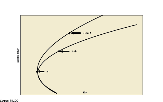
- Combine a hedging portfolio with an active fixed income portfolio and add beta and alpha risk to diversify the overall portfolio. (See the point H+B+A in the chart below.)
 Although solution 1 may work for sophisticated pension funds, it also requires a significant investment in risk monitoring systems and operational systems. It will require managers to abandon traditional thinking about asset classes and instead focus on a more analytical approach to spend the risk budget of the pension fund according to marginal risk/return to the surplus. It also requires extensive knowledge and compliance monitoring to ensure that derivatives are applied correctly to take in risks that are desired and at the same time making sure that no other unwanted risks creep into the portfolio (e.g. counterparty risk).
Given these practical problems, solution 2 may prove to be the next best solution and the most practical way to incorporate alpha and beta opportunities. This is achieved by exploiting the full universe of investment possibilities, rather than being restricted by the chosen benchmark (in this case closely mirroring the liabilities). By determining an ex-ante tracking error versus the customized benchmark, the pension fund can rely on an active manager taking calculated risk – by diversifying strategies – in order to outperform the liability driven benchmark, while avoiding being ‘locked in’ by the same benchmark.
It is worth highlighting that alpha strategies in longduration mandates are not inherently ‘riskier’ than in standard mandates (e.g. euro aggregate mandates). An active fixed-income manager should spend the risk budget in a diversified way, by overlaying the benchmark portfolio with an array of fixed-income opportunities.
Alpha found in different areas of the yield curve as well as outside the base currency can be ‘ported’ on the chosen benchmark and enhance the return of the portfolio. This concept of portable alpha can be explained by a simple observation on yield curve segmentation: whereas the short end of most yield curves is anchored by money market funds looking for investments up to two years, the long end of the yield curve is anchored by institutional investors looking for long term assets to match liabilities. This phenomenon leaves the middle part of the curve largely ‘unanchored’ as there are no natural buyers of this part of the curve. This is where an active fixed income manager can arbitrage segmentation and exploit the steeper roll-down of the curve in the 3-5 year area. This alpha can than be ‘ported’ on the chosen benchmark, whether this is a Libor benchmark or a long duration benchmark is irrelevant.
Inflation and the impact on LDI
The hit on the solvency rate if inflation were to be unconditionally compensated would be gigantic: using break-even inflation rates derived form inflation-linked bonds to form a real yield curve, the average pension fund would take an additional 25-40% hit in the solvency rate. Even though in most cases pension funds have switched to conditional inflation compensation and therefore a nominal framework for hedging liabilities is sufficient, we cannot ignore inflation all together.
Firstly, liabilities will rise in line with real wage inflation, thus raising the overall liabilities to be covered. Secondly, most pension funds will at least strive to (partly) compensate pensioners for inflation and thus will strive for a higher surplus that will allow them to pay out this compensation. The current plans speak of an inflation compensation ‘ambition’ of the pension fund, but this is in our view a rather vague concept and hard to model. In that respect it might be good to look at the UK model, where many pension plans have an explicit upper limit for inflation compensation (most commonly 5%).
In the absence of such specific rules, inflation-linked bonds can fulfill a role in both the hedging portfolio, as well as play a role in adding ‘beta’ risk:
- Inflation-linked bonds provide a direct link with consumer inflation, which has a high correlation with wage inflation. Euro- or even global inflation-linked bonds provide the necessary liquidity and desired correlation with domestic inflation to allocate substantial amounts to this asset class.
- Due to diversification effects in the portfolio, inflation-linked bonds can ‘free up’ risk budget to be allocated elsewhere (e.g. alternative asset classes).
Conclusions
Far from promoting a ‘one-size fits all solution’, we hope to have given you some insights on how we have structured solutions for clients that have opted for an LDI mandate. In our view it is vital to:
Provide input to structure a benchmark that is transparent and adjustable with the client and consultant Evaluate cash flow changes at least on an annual basis and more frequently if events (e.g. takeovers) warrant a review
Exploit the portable alpha concept in full to meet the clients objectives and add value consistently without adding volatility to the pension plan’s surplus.
References
- Asay, Mike; Bhansali, Vineer: Bull Bear Curve Duration, PIMCO Analytics, 2002.
- Bhansali, Vineer: Role of asset managers in asset/liability management of financial institutions
Noten
* The authors wish to thank Alessio Caldarera and the Financial Engineering team at PIMCO, as well as Steve Goldman, Paul Allen and Mike Amey at PIMCO Europe Ltd for their contributions. Pimco Europe Ltd is authorised and regulated by the Financial Services Authority in the UK
in VBA Journaal door Emanuele Ravano, Marc B.M. van Heel
