The role of portfolio optimization
 Portfolio optimization is the current academic standard for determining an investor’s optimal portfolio. By incorporating future return information and the investor’s goal into the optimization problem, it aims to determine the investor’s optimal investment decision. Although incorporating, e.g., transaction costs, expert opinion and liquidity constraints into the optimization problem can make it more realistic, an optimization problem remains a simplification of reality. As a result, optimal portfolios are often unrealistic. Therefore, in practice, investors combine the optimal portfolio with additional information that was not or could not be incorporated into the optimization problem. So, for investors, portfolio optimization does not directly lead to optimal investment decision making, but is a tool that supports it.
Another reason why portfolio optimization can lead to unrealistic portfolios is that optimal portfolios are sensitive to changes in the optimization’s input parameters (Kondor et. al. 2007; Ciliberti et. al. 2007). For example, in mean-variance optimization, optimal portfolios are sensitive to the estimated mean and covariance matrix (Frankfurter et. al. 1971; Michaud 1989; Chopra 1993). Typically, the sensitivity arises because the input is uncertain and, more importantly, because portfolio optimizers push the optimal portfolio towards extremes. Robust optimization approaches such as resampling (Michaud 1998) and Black-Litterman inverse optimization (Bertsimas et. al. 2012) can solve this sensitivity problem. But, also these approaches try to find a portfolio that is optimal in a simplified optimization problem and don’t deal with information that was not or could not be incorporated into the optimization problem.
Portfolios just below the efficient frontier can be completely different from the optimal portfolios on the frontier
What should be the role of optimal portfolios? A good methodology should both solve the robustness problem and serve as a tool that supports optimal investment decision-making. As pointed out in Chopra (1993), portfolios just below the efficient frontier can be completely different from the optimal portfolios on the frontier. In this paper, we show how these near-optimal portfolios can be used in a new methodology for portfolio construction. Our methodology is both more robust and aims to support the investor’s investment decision making.
Near-optimal portfolios
Consider the following simplified example of an investor who can invest in three asset classes: stocks, bonds and private real estate. This simplified example fits with the current low interest rate environment where investors “search for yield” in illiquid asset classes such as private real estate.
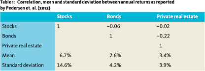 Although illiquid asset classes provide opportunities, they are difficult to model and cannot easily be quantitatively compared to traditional asset classes. The main cause lies in limited data availability and low data quality. For example, for private real estate, the volatility is often underestimated due to appraisal effects (Fisher and Geltner 2000), i.e., real estate properties are valued through appraisals and future appraisals highly correlate with past appraisals resulting in smoothed observations with little volatility. This is also reflected in the statistics in Table 1 as reported by Pedersen et. al. (2012) where the standard deviation of private real estate is low compared to its mean return.
Optimal portfolios typically have unrealistically high allocations to alternative asset classes. See, for example, Figure 1 which shows the mean-variance efficient frontier calculated on the statistics in Table 1. The orange dot denotes the investor’s preferred position on the frontier at 4.5% return. The corresponding optimal portfolio is extreme and consists of 33% stocks, 67% private real estate and holds no bonds. As noted, in this paper, we will show how the near-optimal portfolios just below the frontier can be used to construct a less extreme and more realistic portfolio.
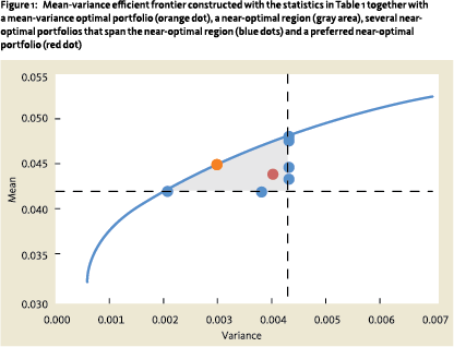 Finding all near-optimal portfolios is done in several steps. Here, we give an intuitive description; the full technical details can be found in van der Schans and de Graaf (2017). First, we start with the optimal portfolio on the efficient frontier as indicated by the orange dot in Figure 1. Then, around this portfolio, we define a near-optimal region by choosing bandwidths around the mean and variance of the optimal portfolio, i.e., the gray area in Figure 1. The idea is that all portfolios in the near-optimal region have a satisfactory risk-return tradeoff and can, especially in the light of the sensitivity, be considered comparable or, at least, acceptable for the investor.
Third, we find a portfolio that is still near-optimal, but is furthest away from the mean-variance optimum (orange dot) in terms of allocation weights. This portfolio can be found with a numerical solver and results in one of the blue dots indicated in Figure 1. It can be shown that all weighted averages of this portfolio and the optimal portfolio remain near-optimal.
Finally, we iteratively continue this process by finding a portfolio that is furthest away from all nearoptimal portfolios, i.e., all weighted averages of the orange and blue dots, found so far. So, the third portfolio is furthest away from all weighted averages of the orange dot and the near-optimal portfolio found in the third step.
The process results in a mean-variance optimal portfolio (orange dot) together with several nearoptimal portfolios (blue dots) of which their weighted average spans the near-optimal region (gray area), i.e., each near-optimal portfolio can be written as a weighted average of the orange and blue dots, and each weighted average of the orange and blue dots is near-optimal. Consequently, we have constructed the near-optimal region.
Near-optimal portfolio construction
Instead of having one optimal portfolio, the region of near-optimal portfolios provides the investor with a whole range of portfolios to choose from. The preferred near-optimal portfolio can be constructed using any quantitative or qualitative information that was not or could not be incorporated in the optimization problem, e.g., liquidity, ESG preferences, transaction cost etc. This portfolio construction process is, similar to the investor’s investment decision making, qualitative and there is not necessarily one best way to do it.
In our simplified example, we select the portfolio from the near-optimal region that is closest to the orange dot in terms of risk and return and has an exposure to private real estate of at most 10%. This results in the portfolio represented by the red dot which consists of 42% stock, 48% bonds and 10% private real estate.
In practice, investors typically impose additional constraints on the optimization problem to force the optimal portfolio towards less extreme allocations. The advantage of the near-optimal region, however, is that it gives insight into the tradeoff that takes place between asset classes and directly shows which alternatives exist to the optimal portfolio.
Robustness of the near-optimal region
Van der Schans and de Graaf (2017) shows that using a near-optimal region results in more robust portfolios. Changing the optimization problem’s input parameters typically has much smaller impact on the near-optimal region than on the optimal portfolio, i.e., most near-optimal portfolios remain near-optimal.
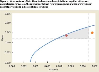
In our simplified example, we illustrate these findings by increasing the volatility of private real estate to 7% and increasing its correlation with stocks and bonds to 0.5. Figure 2 shows the new efficient frontier and near-optimal region. The old optimum now lies outside of the near-optimal region. The proposed near-optimal portfolio consisting of 42% stocks, 48% bonds and 10% private real estate allocation, however, remains near-optimal. One might argue that, obviously, changes made to private real estate have a larger impact on portfolios with a large exposure to private real estate. But, remember that optimizers push portfolios towards extremes and are thus generically expected to be less robust.
 A more realistic example
The methodology can similarly be applied in a more realistic setting with more asset classes. The main difference lies in the construction of the preferred near-optimal portfolio. Consider an investor who can invest in 8 asset classes: government bonds, investment grade bonds, high yield bonds, cash, mortgages, equity developed markets, equity emerging markets, and private real estate, see Table 2 for the describing statistics. Currently, the investor holds a portfolio with 50% government bonds, 40% equity developed markets and 10% private real estate and the investor wants to improve his portfolio by adding the remaining asset classes.
The near-optimal region shows which alternatives exist to the optimal portfolio
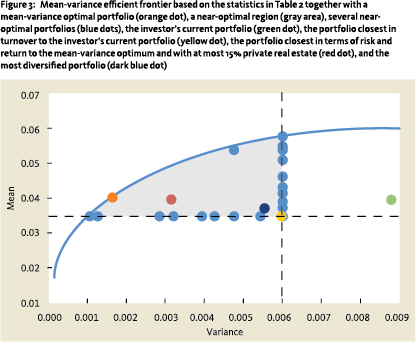
In Figure 3, we constructed the near-optimal region such that it contains portfolios with a return larger than 3.5% and a standard deviation of at most 7.7%. The near-optimal region is spanned by the weighted averages of nearly 50 portfolios. In addition to the describing statistics, Table 2 shows several near-optimal portfolios. In line with Chopra (1993), many near-optimal portfolios have a similar mean and standard deviation but have completely different allocation weights. Also, note that the near-optimal portfolios listed in Table 2 are, by construction, extreme; their purpose is to span the near-optimal region.
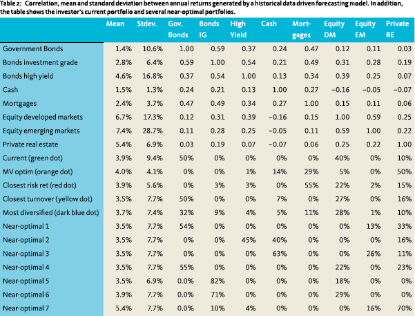 Finding the preferred near-optimal portfolio by manually assigning weights to the near-optimal portfolios in Table 2 becomes harder as more asset classes are added. Also, proceeding as in our previous example does not lead to improvement since it appears that the portfolio with most 15% private real estate which is closest to the mean variance optimum (red dot) contains 55% mortgages. Such a portfolio would not be considered well-diversified and is still unrealistic. With more asset classes, one could start with the investor’s current portfolio (green dot) and look for the nearoptimal portfolio that can be reached with the lowest amount of turnover (yellow dot). In this portfolio, the allocation to developed market equity is decreased by 13% in favor of cash and private real estate. Adding these asset classes brings the investor’s portfolio on the border of the near-optimal region. When the investor is willing to increase the turnover to say 30%, we can search, e.g., for the portfolio that is most diversified over the asset classes (dark blue dot). This portfolio sells 18% of the government bonds and 12% of the equity developed markets and spreads this out between the remaining asset classes. Both these portfolios are realistic options for the investor to consider.
Conclusion
Constructing near-optimal portfolios just below the efficient frontier can have significant added value in portfolio construction. By construction, their risk and return is comparable to the optimal portfolio, but these portfolios can have completely different weights. The constructed near-optimal region can be used to support the investor’s investment decision making. It gives him the possibility to bring in qualitative and additional quantitative information to construct realistic portfolios with favorable risk-return tradeoffs.
References
- Bertsimas, D., V. Gupta and I. Ch. Paschalidis, 2012, Operations Research, vol. 60 nr. 6: 1389-1403.
- Chopra, V. K., 1993, Improving Optimization, The Journal of Investing, vol. 2 nr. 3: 51-59.
- Ciliberti, S., I. Kondor, and M. Mézard, 2007, On the feasibility of portfolio optimization under expected shortfall, Quantitative Finance, vol. 7 nr. 4: 389-396.
- Fisher, J. D., and D. Geltner, 2000, De-lagging the NCREIF index: transaction prices and reverse-engineering, Real Estate Finance, vol. 17 nr. 1: 7-22.
- Frankfurter, G. M., H. E. Phillips, and J. P. Seagle, 1971, Portfolio Selection: The effects of uncertain means, variances, and covariances, Journal of Financial and Quantitative Analysis, vol. 6 nr. 5: 1251-1262
- Kondor, I, S. Pafka and G. Nagy, 2007, Noise sensitivity of portfolio selection under various risk measures, Journal of Banking and Finance, vol. 31 nr. 5: 1545-1573.
- Michaud, R. O, 1989, The Markowitz Optimization Enigma: Is ’Optimized’ Optimal?, Financial Analysts Journal, vol. 45 nr.1: 31-42.
- Michaud, R., 1998, Efficient Asset Management: a practical guide to stock portfolio management and asset allocation, Financial Management Association Survey and Synthesis, Boston, HBS Press.
- Pedersen, N., A. Tiwari, and A. Hoffmann, 2012, Modeling the risk characteristics of real estate investments, PIMCO working paper.
- Schottle, K., R. Werner, 2006, Towards reliable efficient frontiers, Journal of Asset Management, vol. 7 nr. 2: 128-141.
- Van der Schans, M., de Graaf, T., 2017, Robust optimization by constructing near-optimal portfolios, Ortec Finance methodological working paper, nr. 2017-02.
Note
- Martin van der Schans is researcher at Ortec Finance.
in VBA Journaal door Martin van der Schans
