
INTRODUCTION
 After a period of low and even negative interest rates in 2020 and 2021, rates soared in 2022 and have remained high. In this article we want to address several topics. First, we illustrate what the impact on expected returns has been with a Capital Market Assumptions (CMA) model. One of the main observations is that the risk premium of equities versus bonds has declined. The second section provides explanations as well as justifications. In short, a lower equity risk premium (ERP) is not just a reflection of equities being expensive, but is justified as bonds have become riskier relative to equities. Finally, we show the extent to which the change in interest rates and CMAs leads to different ‘optimised’ portfolios. The rise in yields and the lower ERP result in more fixed income assets and fewer equities in portfolios in 2024 than in 2020. Optimised fixed income portfolios, from an asset only perspective, consist of cash and spread products, but do not contain any government bonds. That holds for both 2020 and 2024. Furthermore, the rise in riskfree yields has resulted in IG Corporates gaining a place in the spread portfolios at the expense of riskier spread products such as emerging market debt (EMD) and high yield. Within equities, developed markets have become less attractive compared to emerging markets due to increased volatility. Finally, lower risk portfolios have experienced an increase in expected return benefitting from higher yields, while higher risk portfolios have become more diversified, as differences in expected returns between (fixed income and equity) asset classes have become smaller.
IMPACT ON CAPITAL MARKET ASSUMPTIONS
 METHODOLOGY: CMA MODEL
Several methodologies for Capital Market Assumptions (CMA) models are used in the financial sector. A first distinction is between models that create absolute returns per asset class and models that generate risk-premia per asset class versus cash; so absolute versus relative. A second distinction is between econometric approaches that use historic regression to determine the return forecast and marked-implied approaches linked to prevailing and forward looking market data.
The Columbia Threadneedle CMA model adopts an absolute return perspective combined with a marked-implied approach. The model generates expected returns and volatilities on a monthly basis for 22 individual asset classes on a five-, tenand fifteen-year horizon. It incorporates the latest consensus expectations regarding economic growth and the forward paths for inflation and interest rates. Due to multiple horizons, the CMA model can be used for different objectives: the 5-year CMAs are used for more tactical tasks such as updating annual investment plans, while the 15-year CMAs are used as input for asset and liability management studies. The monthly updates provide insight into the impact of prevailing market developments.
The focus in this article is on the five-year CMAs.
To provide some colour on the CMA model, the methodology for several assets is outlined.
The expected returns for risk-free euro governments bonds are produced based on prevailing bond yield levels and forward paths for the interest rates of the various governments over the next 15 years. This results in a ‘yield’ return, a ‘roll down’ return, and a ‘price’ return for each calendar year.
Expected returns for spread products are modelled similarly to government bonds. Income, carry and price returns are calculated for different calendar years based on prevailing interest rates, expected interest rate paths and durations. The only addition is that the interest rate path consists of a separate path for the risk-free interest rate component (based on the forwards) and one for the spread component (moving from the current level to the long-term average at that time). Discounts are also applied for credit losses (based on long-term statistics from credit rating agencies per rating letter).
IN ONE WAY OR ANOTHER, THE EXPECTED RETURNS OF ALL ASSET CLASSES ARE LINKED TO INTEREST RATES
 The expected returns for equities are composed of income (linked to dividends and buybacks) and expected earnings growth (linked to economic growth assumptions and inflation swaps). An adjustment is also made for hedging currency risk. On a euro-hedged basis, this currently results in a markdown because USD rates are higher than EUR rates. Finally, an sadjustment is made for valuation. This component can be positive or negative, and its contribution is theoretically zero in the long run. To assess valuation we look at the price/earnings (P/E) ratio based on expected earnings and compare this to our long-term P/E target (modelled on volatility and forward interest rates).
Additionally, for several asset classes the expected returns are created via ‘mapping’ of other asset classes. For instance, the returns for private equity, real estate and infrastructure are based on those for developed markets equities plus or minus a fixed premium or discount. For real estate and infrastructure an adjustment is also made for the higher interest rate sensitivity compared to equities. This is based on forward interest rates and an estimated sensitivity – a projected interest rate increase will lead to a lower return and vice versa.
In one way or another, the expected returns of all asset classes are slinked to interest rates. For fixed income the relationship is obvious. For others such as equities and real estate, interest rates affect valuation. Some asset classes have an indirect link via ‘mapping’ to assets with a link to rates. For alternatives such as Commodities and Catastrophe Bonds, the path for interest rates has a direct link with the collateral return component.
THE IMPACT OF HIGHER INTEREST RATES ON CMAS
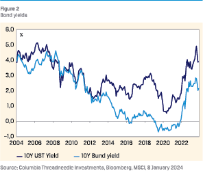
 As outlined, to varying degrees interest rates affect the expected returns of all asset classes. Our CMA model has been live since May 2020. At that time bond yields traded at historical lows: the 10-year Bund at roughly –0.5% and the 10-year US Treasury (UST) at around 0.5%. Markets were pricing in a modest increase in yields. That combination led to negative expected returns for euro government bonds.
The expected return for euro core government bonds was about –1% on a five-year horizon. By 2021, the expected return for global high yield also turned negative, driven by a decline in HY spreads and higher FX hedging adjustments, as well as the low risk-free rates. Lower spreads reduce expected returns via lower income, but also via expected negative indirect returns as spreads are assumed to eventually rise to neutral levels. At that time, expected returns for developed markets equities were still in positive territory at roughly 4%. The premium of equities versus euro core government bonds was no less than 5% at that time, according to the CMA model.
Since then, a lot has changed. Interest rates have risen significantly since early 2022, triggered by a combination of the inflation shock caused by the Covid-19 pandemic and the Russian invasion of the Ukraine, and the subsequent massive tightening cycle by the US Federal Reserve and the European Central Bank. The 10-year UST yield rose by 4.5%-point to 5% in 2023 and the 10-year Bund yield rose by 3.5%-point to close to 3%. Since then yields have eased back a little, but are still trading significantly higher than in 2021 at 4.1% and 2.2% respectively, as at January 2024.
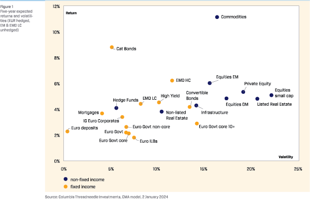
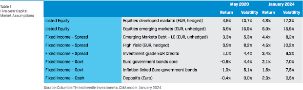
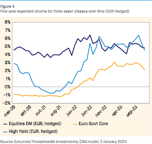 Fixed income CMAs have changed substantially too, as illustrated in the chart. The five-year expected return for euro core government bonds has increased to 2.6%, as of January 2024, and the expected return for high yield – also supported by the subsequent rise in spreads – has increased to 5.4%. The expected return for equities has remained fairly stable and currently amounts to 4.9%. However, the components of the expected return did change: inflation expectations increased, expected economic growth decreased, and the valuation adjustment turned more negative as prices increased and yields rose.
THE RISK PREMIUM OF EQUITIES HAS SHRUNK CONSIDERABLE COMPARED TO EURO GOVERNMENT BONDS
In short, the impact of rising interest rates on CMAs has been an increase in expected returns for fixed income asset classes (and especially spread products), while equities remained fairly stable. Consequently, the risk premium of equities has shrunk considerable compared to euro government bonds – with the expected return of high yield even higher than that of developed markets equities.
LOW EQUITY RISK PREMIUM
As outlined above, the equity risk premium has tightened significantly since mid-2022. This can be illustrated in several ways. A simple measure is by taking the difference between the earnings yield (which is the inverse of the P/E ratio1) on equities and bond yields.2 A more sophisticated method is to take the difference between the five-year expected return of developed markets equity and that on euro core government bonds from the CMA model. Both methods provide a similar message: the ERP is historically low.
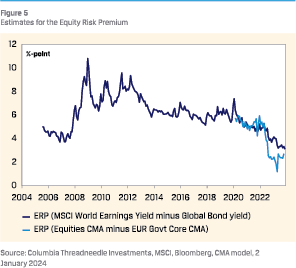 We have several explanations as well as justifications, for the low ERP. Explanations merely describe how the EPR declined, while justifications also make the case for why investors would be willing to accept a lower ERP.
EXPLANATION 1: HIGHER INTEREST RATES
As explained above, the rise in interest rates led to higher expected bond returns and subsequently a lower ERP.
EXPLANATION 2: HIGHER EQUITY PRICES AND HIGHER EQUITY VALUATIONS
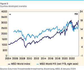
Although equity markets initially reacted negatively to the massive monetary tightening cycle in 2022, equity prices have since recovered. P/Es based on expected earnings have risen and are now at levels similar to early 2022. The CMA model indicates that P/Es are too high, with the target P/E dropping as a result of higher yields. In other words, equities are too expensive, which is reflected in a negative valuation component in the CMA model, resulting in a lower ERP.
These explanations imply that equities are less attractive versus bonds than they were two years ago, and investors should reduce their exposure.
We can also suggest more than one justification for the apparently low ERP that would suggest equities are more attractive than presented on the basis of the ERP.
POSSIBLE JUSTIFICATION 1: REDUCED EQUITY RISK COMPARED TO BONDS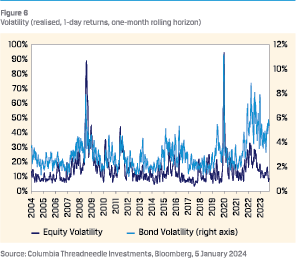
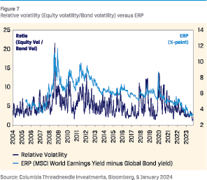
Equities may have become less risky relative to bonds, thereby requiring a lower risk premium. Several indicators support this.
First, although equity volatility rose markedly from mid-2021 during the inflation shock and tightening cycle, it has since come down and is historically low. Bond volatility also rose markedly but remained high. As a result, equity volatility has declined significantly compared to bond volatility. That justifies a lower ERP.
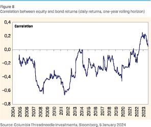
 Second, while government bonds have usually provided a hedge against equity risk at times of economic crisis, they also took a beating during the inflation shock of the past couple of years. This meant the correlation between equity and bond returns flipped from negative to positive. So, with less diversification potential, the attractiveness of government bonds has decreased from a portfolio perspective. That also justifies a lower ERP. Although inflation has now declined substantially, inflation risks remain high as geopolitical tensions are far from gone. As real assets provide a better hedge against inflation than nominal assets, a low ERP might be interpreted as an insurance premium.
 Third, government bonds with a high credit rating (AAA-AA) are often labelled risk-free assets. However, credit risk is once again becoming an important factor for sovereigns. Sovereign debt has been rising for years, both in emerging and developed markets. This trend will continue in coming years, according to the IMF. The consensus also assumes significant fiscal deficits in the coming years in the US, the eurozone, the UK, Japan and China. The supply of government bonds will therefore increase, as will credit risk. Both factors have un upward effect on interest rates. If bond yields rise due to an increase in the credit risk component, that would justify a lower ERP as it would signal that bonds have become riskier, not that equities have become more expensive.
SO, LOOKING AT VOLATILITY, INFLATION RISK, DIVERSIFICATION AND CREDIT RISK, GOVERNMENT BONDS HAVE BECOME RISKIER VERSUS EQUITIES IN RECENT YEARS, THEREBY JUSTIFYING A LOWER ERP
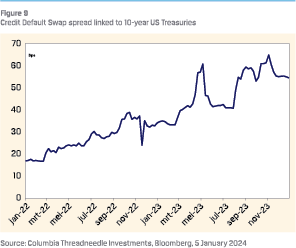 Increasing credit risk applies more to the US than the eurozone. Debt/GDP levels in the eurozone are expected to rise less (or even decrease in some countries) than the US. Also, credit default swap (CDS) spreads linked to US government bonds have risen (the 10-year US CDS rose from around 20bps in early 2022 to 55bps now), while CDS spreads in the eurozone have remained fairly stable (the 10-year German CDS trades at 25bps).
So, looking at volatility, inflation risk, diversification and credit risk, government bonds have become riskier versus equities in recent years, thereby justifying a lower ERP.
POSSIBLE JUSTIFICATION 2: ARTIFICIAL INTELLIGENCE
As stated, one explanation of the declining ERP was the rise in equity prices. The rally was mainly driven by IT stocks, particularly by the Magnificent Seven, which in turn was driven by artificial intelligence (AI). That might also be a justification as well as an explanation. The argument is that AI will lead to huge productivity improvements and thereby additional EPS growth. So, while equities might seem expensive based on current earnings, the valuation could be justified from a more forwardlooking perspective. However, our CMA model uses growth forecasts up to five years (Bloomberg consensus and IMF forecasts) and EPS forecasts up to three years, and still suggests that equities are expensive. So, for the AI justification to be valid, the markets’ assumption would have to be that the AI productivity boost is mainly expected on horizons in excess of three to five years. That might well be the case – according to a recent article by The Economist, the AI revolution will take time.3
IMPACT ON ASSET ALLOCATION
In this final section, we will illustrate to what extent the change in interest rates and CMAs leads to different ‘optimised’ portfolios. We have used CMAs from 2020 and 2024, and the analysis is simplistic, using only eight liquid asset classes: equities, spread products, government bonds and cash. Furthermore, it is an ‘asset only’ perspective. So, the risk measure is the volatility of the portfolio, and not for instance a tracking error versus liabilities. The goal of the optimization is to find optimal asset allocations that deliver the highest expected returns, for given levels of volatilities.
The starting point is unconstrained mean variance optimisation (MVO) introduced by Markowitz in the early 1950s. In the MVO process, the expected returns and volatilities, together with the historical correlations are used. This classical optimization has several well-known shortcomings. No consideration of estimation error and sensitivity to the inputs are the main concerns. This can result in ‘error maximization’, since it overweights assets with positive error and underweights ones with negative error. The cornered solutions do not offer adequate diversification within the portfolio, and likely lead to large transactions in the following periods. Besides, it is undesirable that even slight changes in CMAs can lead to significant differences in optimal portfolios.
To mitigate the drawbacks of MVO, constraints are often added such as imposing lower and upper boundaries for each asset class. Another method is to take uncertainty in input parameters into account, such as robust optimisation (RO), which was introduced by Ben-Tal and Nemirovski [1998].4 RO provides one single optimal solution that is robust to all possible scenarios within the uncertainty set, rather than a set of solutions for different scenarios, as in stochastic optimization. Unlike in MVO, where the inputs are traditional CMA forecasts, such as expected returns and volatilities, the inputs for RO are the uncertainty sets including these point estimates. That is why RO is also considered to be optimal for the worst-case objective function, as even if the true value takes its worst possible value within the uncertainty set, the allocation remains optimal (Fabozzi et al. [2007]5). What RO effectively achieves is the avoidance of corner solutions and better diversification of assets than the classical MVO.
In terms of estimation error, it is widely believed that most of the estimation risk in the optimization process comes from the estimation error in expected returns, and not in expected risk. Although returns and risks change over time, risk is more persistent. Besides, portfolio managers often have higher confidence in risk estimation than in return estimation. For this reason, we focus on the estimation error in our CMA returns. There are different forms of uncertainty sets. We use a quadratic uncertainty set which is frequently used in financial literature.
2 n n n n l – – X # – ^
with µ the expected returns, n the estimated expected returns, Ω the covariance matrix of uncertainty in mean return (or uncertainty matrix), and κ the level of uncertainty.6
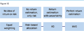 We will not further dive into mathematics. Practically speaking, if κ or Ω are small, the robust portfolio will be similar to MVO solutions (a small estimation error implies a high confidence in estimated returns). If κ or Ω are large (a large estimation error implies less confidence in estimated returns) then the optimal solution can deviate significantly from the MVO, and will converge more towards risk-based portfolio allocations such as risk-parity. Robust portfolio allocation is essentially a weighted average of risk-based allocation and mean-variance allocation (Perchet et al. [2015]7). Which portfolio optimisation method to choose depends on the confidence of the estimation.
Different Ω estimation methods are shown in different literatures. Yin and Perchet [2019]8 suggests Ω to be the diagonal part of the asset covariance matrix Σ.
We take this as a starting point with a few modifications. We use volatilities based on monthly returns over the past 15 years. We then calibrate Ω values by several factors, as volatility alone doesn’t capture the complete picture in our opinion. Several factors and perspectives are used to compose Ω for individual assets classes:
- . In line with literature, the variance is used as a starting point and main building block for Ω;
- Then, an adjustment is made for the importance of income return. In our opinion, the return of asset classes for which the total return is mainly driven by indirect return and not direct return is more difficult to predict. So, the Ω component for an asset class such as commodities which is mainly price driven will be adjusted upward versus that of an asset class such as corporate bonds which to a large extent are driven by income in the long run;
- The third factor is skewness, a factor not captured by variance. For asset classes with a significant negative skew (such as catastrophe bonds), the Ω component is also increased.
Finally, a limit is applied. The Ω component cannot be higher than assets’ expected returns. It makes little sense if the estimation error is higher than the estimation itself.
Once Ω is set, κ will have the total level of uncertainty within requirements. We do not want κ to be too high, as otherwise the optimal portfolio allocations will be too conservative mirroring that of risk-based allocations, and too much performance will be sacrificed.
The results are shown in the charts above. The main observations are:
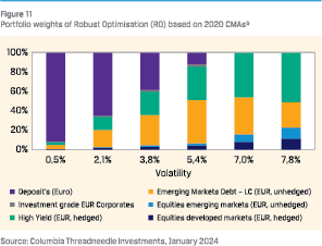 Contrary to MVO portfolios (which are not shown in this article) where the portfolio with the highest risk simply consists of the one asset with the highest expected return, the RO portfolios are more diversified. Adding uncertainty to expected returns results in less corner solutions. The assets of the portfolio with the highest risk are not just equity related but also fixed income related. Increased diversification is also observed within the equity portfolio.
- Moving from low-risk (left) to high-risk portfolios (right), the portfolios first include cash, then spread products (EMD and to a lesser extent high yield), and finally equities. None of the MVO portfolios (2020 nor 2024) contain government bonds. This is in contrast to pension fund portfolios with large government bond holdings as matching instruments. From an asset only perspective, however, these are less attractive apparently. The explanation being that the return per unit of risk is low compared to that of spread products and certainly versus cash.
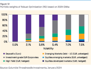 The rise in yields and the lower ERP are reflected in the 2024 mixes that on balance contain more fixed income products and less equities. For instance, riskier RO 2020 portfolios assign a 24% weight to equities (developed and emerging), whereas the riskier RO 2024 portfolios assign just 10% to equities.
- Furthermore, in the low risk and fixed income dominated RO portfolios cash gets an even higher weight in 2024 than in the 2020 mixes. With money market rates moving from negative territory to positive territory while having a very low volatility, money market products have become more attractive.
- The RO 2024 portfolio includes a significant portion of IG Corporates. This is due to the significant rise of risk-free rates as this asset class did not appear in the 2020 portfolios. Also, the use of an uncertainty set is relevant as the asset class was not part of the MVO 2024 portfolios.
- The riskier 2024 CMA RO portfolios contain more asset classes (five or six) than the riskier 2020 CMA RO portfolios (four assets). As differences in expected returns between (fixed income and equity) asset classes have become smaller by 2024, the 2024 high risk portfolios have become more diversified.
AS DIFFERENCES IN EXPECTED RETURNS BETWEEN (FIXED INCOME AND EQUITY) ASSET CLASSES HAVE BECOME SMALLER BY 2024, THE 2024 HIGH RISK PORTFOLIOS HAVE BECOME MORE DIVERSIFIED
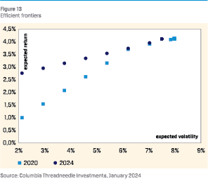 We have also plotted the RO efficient frontiers for 2020 and 2024. The main observation is that in 2024 the low-risk portfolios have a much higher expected return than in 2020. The explanation is straightforward: low risk portfolios are dominated by fixed income, and the expected return on fixed income assets has risen considerably since 2020. Expected returns for high-risk portfolios have not changed much.
We recognize that robust optimization is not a universal remedy for portfolio optimization, but the results provide insight. To summarise, the impact of higher interest rates on asset allocation is:
- More fixed income assets and fewer equity assets in portfolios in 2024 than in 2020;
- Fixed income portfolios consist of cash and spread products but do not contain any government bonds. That holds for both 2020 and 2024;
- Furthermore, the rise in risk-free yields has resulted in IG Corporates gaining a place in spread portfolios at the expense of riskier spread products such as EMD and High Yield;
- Within equities, developed markets have become less attractive than emerging markets due to increased volatility;
- Also, lower risk portfolios have experienced an increase in expected return;
- Finally, higher risk portfolios have become more diversified, as differences in expected returns between (fixed income and equity) asset classes have become smaller.
As a final remark, we want to reiterate that portfolio optimisation is only intended as an illustration. In reality, outcomes can differ significantly versus the above results depending on CMAs, assets classes used, bandwidths per asset class, optimisation methods, risk budgets, and possible liability matching objectives. However, we believe it provides useful insight into the consequences of the rise in interest rates.
Notes
- We have used the P/E of the MSCI World Index, based on estimated earnings for Fiscal Year 3. FY3 earnings are more stable than FY1 earnings.
- We have used the yield of the Bloomberg Global Agg Treasury index.
- https://www.economist.com/finance-and-economics/2024/ 01/07/what-happened-to-the-artificial-intelligenceinvestment-boom
- Ben-Tal, A., and Nemirovski, A., 1998, Robust convex optimization. Math. Oper. Res. 23, 769–805.
- Fabozzi, F.J., Kolm P.N., Pachamanova D.A., and Focardi S.M., 2007, Robust Portfolio Optimization. The Journal of Portfolio Management, Vol. 33, No. 3 (Spring), pp. 4048.
- The scaled sum of the squared spreads between the true expected returns and the estimated returns, should be smaller or equal to “κ” ^2, with the scaling factor the inverse of the covariance matrix of the estimation errors.
- Perchet, Lu, Carvalho, and Heckel, 2015, Insights into Robust Portfolio Optimization: Decomposing Robust Portfolios into Mean-Variance and Risk-Based Portfolios.
- Yin, and Perchet, 2019, A Practical Guide to Robust Portfolio Optimization
- One consequence of the fact that RO portfolios are more diversified than MVO portfolios is that the volatility of the highest risk RO portfolios is much lower (8%) than that of the highest risk MVO portfolios (15.5 %). Hence, the difference in scales of the charts.
in VBA Journaal door Jitzes Noorman and Shengsheng Zhang